Draft for Information Only
Content
Integration
IntegrationIntegration is concerned with the finding of the antiderivative of a function. Integral of a functionSimilar to differentiation, integral is the result function of the integration, but the function to be integrated is named integrand. As in many daily life problems, knowing what is the effect of the integrand with respect to the variable of integration within an interval of an independable variable is also a very common interest. For example a function f : 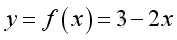
Graph of the function is 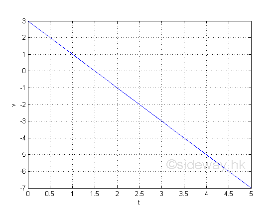
The graph gives a
picture of the independable variable x on the function y.
When x=1; y=1; and when x=2; y=-1. And from the graph, the value of y decreases
as the value of x increase. The graph can only give the exactly value of y
according the value of the independable variable x and there is no information
on what is the effect of y with respect to x within an interval of x. The total effect of y with respect to x within an interval of x can be obtained by summing up all the individual effects of y with respect to x in each infinitesimal interval element along the interval of x. When considering a small infinitesimal interval element Gx of the independence variable x, the total effect of y with respect to x within this small infinitesimal subinterval element can be approximated by rectangle of infinitesimal width at the point of consideration. For example, considering a small interval, 0.5 of the independence variable with a fixed small infinitesimal subinterval element Δx, the calculated results of some typical total effects at points of considerationare:
From the table, the variation of ∑yiΔxi in relation to Δx is obtained. According to the calculated results, the value of ∑yiΔxi varies on both Δx and x. The reduction of Δx can also reduce the value of ∑yiΔxi and values above the x axis is positive while values below the x-axis is negative.. Therefore ∑yiΔxi is not a constant but a function of Δx and x. Since ∑yiΔxi is equal to zero when Δx=0 and the variation of ∑yiΔxi is reduced as Δx becomes small, the value of ∑yiΔxi as Δx approaching 0 can be evaluated by its limit. This type of limit is named integral and the notation is: 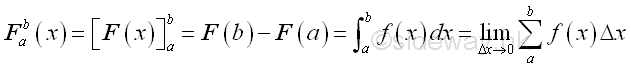
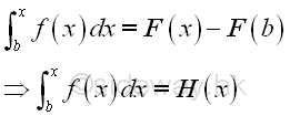
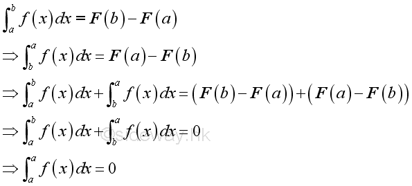
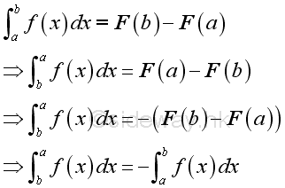
Since the integral is defined as F(b)-F(a) at which a<b, the sign of the integral should be reversed if a>b 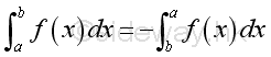
And from the table, the integral of the integrand f at an interval of [a,b], when a=1 and b=1.5 are as following: 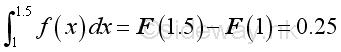
and when a=2 and b=2.5 are as following: 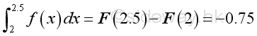
Although the duration is equal to 0.5 for both x=1 and x=2, the total effects on both situation is difference. The integral of function y at the interval [1,1.5] is equal to 0.25 while the integral of function y at the interval [2,2.5] is equal to -0.75. IntegrationInstead of using an numeric value to find the value of the integral of the function f at the interval [a,b], the ∑yiΔxi can be expressed in the form of Δx and x with n infinitesimal interval elements between the interval [a,b], Imply 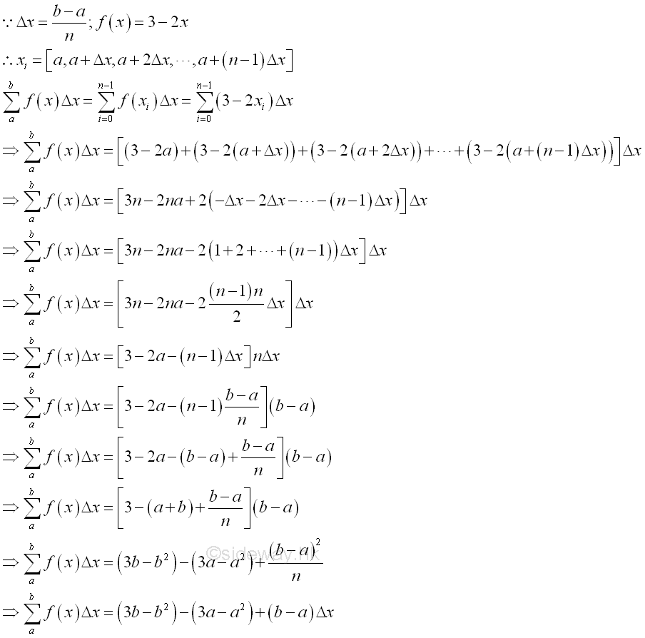
And the integral of the function f is: 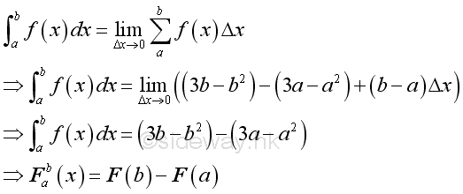
Therefore when Δx approaching 0, the integral of the function y is a function of a and b only. And when the interval of x =[1,1.5], F(b)-F(a)=0.25; and when the interval of x =[2,2.5], F(b)-F(a)=-0.75 as before. From the integral, a more clear picture of what is the total effect of y with respect to x within an interval of x is obtained. Geometrically, integration is usually refered as a method to determine the area under a curve. The definite integral F of the function f(x) on interval [1,1.5] can be expressed as 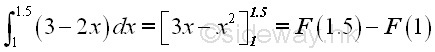
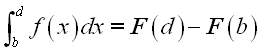
And the definite integral F of the function f(x) on interval [2,2.5] can be expressed as 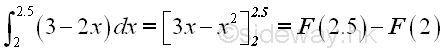
IntegralFor a given function f, if the function f is continuous and defined on an interval [a,b], the function f is integrable on the interval [a,b]. The interval of the function can be divided into finite subintervals. let n be the numer of equal subintervals and Gx be the length of the subinterval. Points on the interval [a,b] of the independable variable is [x0=a, x1=a+Δx, x2=a+2Gx, ..., xi=a+iΔx, ..., xn=a+nΔx=b]. In every subinterval, there are lower and upper subinterval boundries. Consider the ith subinterval, when the subinterval is infinitesimally small, the function f(x) has a minimum and a maximum on the subinterval boundries. Let f(i) be the average value of function f(x) in the ith subinterval, f(iu) be the maximum value of function f(x) in the ith subinterval, and f(il) be the minimum value of function f(x) in the ith subinterval. Therefore the actural total effect of function f(x) with respect to x in the subinterval is Fi =f(i)Δx, the maximum approximation of the total effect of the function f(x) with respect to x in the subinterval is Fu =f(iu)Δx, and the minimum approximation of the total effect of the function y with respect to x in the subinterval is Fl =f(il)Δx. Imply the 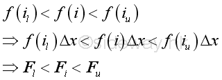
If the number of subintervals is unlimited, there alway exist a number n such that for all subintervals the difference between the upper limit and lower limit of the function f(x) in a subinterval can be less than a selected number. Imply at the ith interval 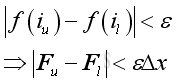
Therefore the lower FL , the upper FU , and the actural F sums of function f(x) on the interval [a,b] are 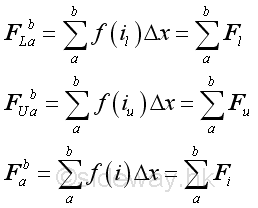
Similarly, the sums are 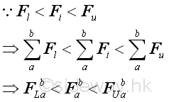
If the number of subintervals is unlimited, there alway exist a number n such that for all subintervals the difference between the upper limit and lower limit of the function f(x) in a subinterval can be less than a selected number. Imply at the interval [a,b] 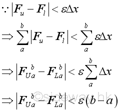
Since function f(x) is continuous on the interval [a,b], the variation of the lower FL and the upper FU on the interval [a,b] has a common limit. If the number of subintervals is unlimited, there alway exist a number n such that the difference between both the lower FL and the upper FU and the actual value F can be less than a selected number. In other words, F is the limit of the lower FL and the upper FU . Let xi be the general term of ith point with subinterval Δx, Imply 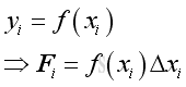
Therefore, 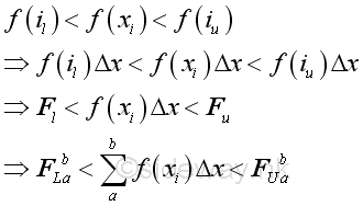
Therefore for a function f that is continuous and defined on an closed interval [a,b], the function is integrable on the interval, that is the following limit exists, Since F is the limit of the lower FL and the upper FU , Imply 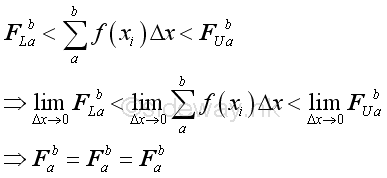
Definite IntegralThis type of limit is called definite integral and the notation is:
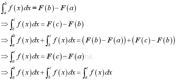
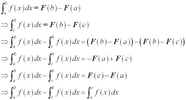
The definite integral is the limit of the summation of function y in the closed interval [a,b]. A definite integral involves the difference between the value of the integral at its upper limit b and the value of the integral at its lower limit a. Therefore a definite integral is also a function of a and b The dx is the infinitesimal value of variable at which the intergration with respect to and to which the limit taken as approaching zero. As shown in the example, the summation of the function can be positive, negative, and zero, depending on the function on the closed interval. The solution of an definite integral is the difference between two indefinite integral. Indefinite integral is the antiderivative of a function, the indefinite integral always involves a constant of integration and a family of antiderivatives can be obtained by adding different constants. But a definite integral does not involve a constant of integration because this is a net value between the upper and lower limits and the constant of integration will be cancelled out during calculation. Some rules of limits of integration are
Indefinite IntegralThe indefinite integral of a function does not have finite values of both upper and lower limits as in definite integral. The indefinite integral is also called an anti-derivative. The indefinite integral of a function f(x) is the general solution of the anti-differentiation of the function f(x). In other words, finding the indefinite integral of a function f(x) is to determine what function can be differentiated in order to get the function f(x). The notation of an indefinite integral is 
From the above example, the integral of the function can be obtained by a reverse differentiation process, that is: 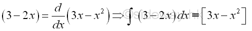
Since the derivative of a constant is zero, any constant can be added to the solution of the anti-differentiation process and the corresponding results are still the integral of the integrand. Therefore in general, the anti-derivative of a integral is a family of non-unique solutions, and these anti-derivatives all differ by a constant, the constant of integration. For example: 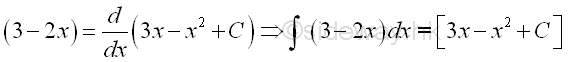
In general: 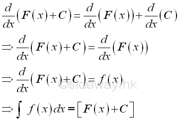
Since the difference of the solution set of anti-derivative is a contant only, for convenient, the indefinite integral can be expressed as: 
where C is an arbitrary constant, the constant of integration. And this is why an indefinite integral is called an ant-derivative Reference to the above example, the definite integral of two closed interval can be rewritten by twe sets of variables as:
If the upper limit c and d are variables then the integral is:
As in the example, these two integrands are integratable at a and b also, and when the upper limits change to a variable, they become indefinite integrals with difference lower limit references, imply.:
Imply the difference between two indefinite integral is always a constant: 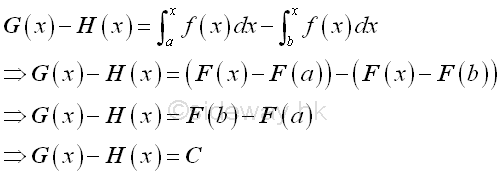
Therefore the general format of an indefinite integral can be expressed as:
where C is an arbitrary constant, the constant of integration. And F(x) is the integral used as in the definite integral. Integration and DifferentiationAccording to the above example, integration is the process of function summation over a closed interval by making the subinterval approaching zero.
Consider a small subinterval, imply 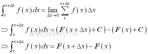
The integral is total effect of function f(x) with respect to x over the duration Δx. And as Δx approaching zero, the integral becomes the intantaneous effect of function f(x) with respect to x. 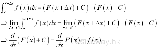
The average effect of function f(x) with respect to x over the duration Δx is therefore equal to . 
In other words as Δx approaching zero, the average effect of function f(x) with respect to x over the duration Δx is also equal to the rate of change of function F at x, Imply 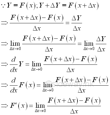
Therefore when Δx approaching zero and there is only one subinterval, the derivative of F(x) is equal to f(x), Imply 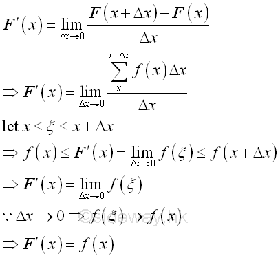
Therefore the indefinite integral of function f(x) is F(x) and the derivative of function F(x) is f(x). Since the difference between any two indefinite integrals of the function f(x) is a constant, imply: 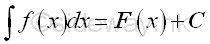
Therefore integration can be considered as the reverse process of differentiation. Indefinite Integral & definite IntegralFor a function f(x), the indefinite integral of a function with a upper limit variable x is
And the differention of the F(x) is 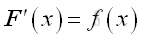
Imply the constant of integration of a definite integral is depending on the lower limit a as the Δa approaching zero, that is 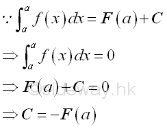
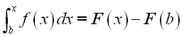
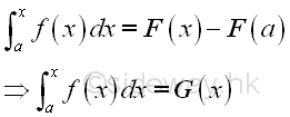
Therefore the indefinite integral of a function with a upper limit variable x can be expressed as: 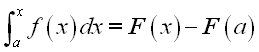
And the definite integral of a function with a upper limit b can be expressed as: 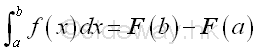
Or in a more convenient format: 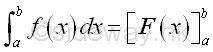
Successive IntegrationSimilar to differentiation, successive integration can also be applied to a function. But a constant of integration is induced automatically after integrating the function each time. For example, the first indefinite integral of a function y=-2 is equal to 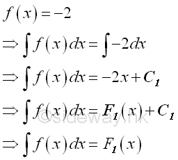
From the first indefinite integral, the total effect of the function f(x) with respect to x is a linear function of x plus a constant of integration C1. The second successive indefinite integration of the function is 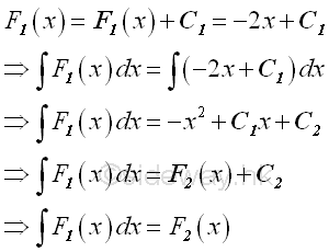
From the second indefinite integral, the total effect of the first integral of the function f(x) with respect to x is a second degree polynomial function of x plus another constant of integration C2. Let C1=3; C2=0, imply 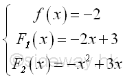
Assumed the mentioned function f is the instantaneous acceleration as a function of time x. Then the first integral is the instantaneous velocity as a function of time x. The second integral is the distance as a function of time x. And higher integrals can be obtained by repeating the integration process , i.e. third integral by taking the integral of the second integral... etc ©sideway ID: 111000017 Last Updated: 11/4/2011 Revision: 2 Ref: References
Latest Updated Links
  Nu Html Checker Nu Html Checker  na na |
 Home 5 Business Management HBR 3 Information Recreation Hobbies 8 Culture Chinese 1097 English 339 Reference 79 Computer Hardware 249 Software Application 213 Digitization 32 Latex 52 Manim 205 KB 1 Numeric 19 Programming Web 289 Unicode 504 HTML 66 CSS 65 SVG 46 ASP.NET 270 OS 429 DeskTop 7 Python 72 Knowledge Mathematics Formulas 8 Algebra 84 Number Theory 206 Trigonometry 31 Geometry 34 Calculus 67 Engineering Tables 8 Mechanical Rigid Bodies Statics 92 Dynamics 37 Fluid 5 Control Acoustics 19 Natural Sciences Matter 1 Electric 27 Biology 1 |
Copyright © 2000-2024 Sideway . All rights reserved Disclaimers last modified on 06 September 2019
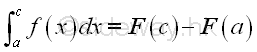 and
and
 and
and