
|
Draft for Information Only
Content
Continuity of Function
Continuity of FunctionContinuity is the large concern in studying the instantaneous change of a function. One of the important application of limit is the determination of the continuity of a function. Graphically, the graph representing a continuous function is a continuous curve with no discontinuity like holes, gap or jumps on the graph. Mathematically, a function is said to be continuous if all functional values of a function are changed continuously as the value of the continuous independent variable is varied continuously along the number line within the domain of the independent variable. In other words, the functional values of the function for every point on the domain of the function should be defined, the limits of the function when taking limit at each point in the domain of the function always exist, and the limits of the function at any point in the domain should equal to the functional value at the point. Imply 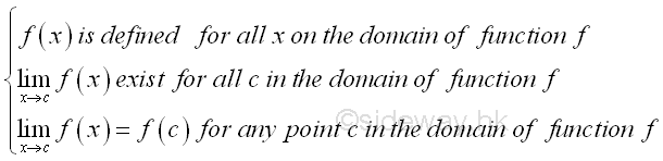
These criterias can also be used to determine the continuity of function at any point xo in the domain. Imply 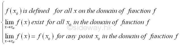
Epsilon-Delta Limit
The continuity of function at a point can also be expressed in terms of epsilon and delta according to the Epsilon-Delta limit definition to examine the neighborhoods of a point in the domain of the function. For example, a continuous curve on the graph is used to represent a function f(x) which is continuous on the domain of the function. The continuity of a point p with coordinates (c,f(c)) on the graph is being examined. By observing the curve segment around the functional value f(c) with upper and lower boundaries located at a distance of a small quantity ε from the functional value f(c). There are always a pair of corresponding boundaries around the independent varible c located at a distance of a small quantity δ' and δ from independent varible c accordingly. Let δ'>δ where in this case, δ' is the lower boundary and δ is the upper boundary. The continuity of the line segment at point p can be determined by examining the functional value at x=c, if the line segment is continuous at c, the function value f(x) should be defined and is equal to f(c), i.e. f(x)=f(x). Besides, if the line segment at c is continuous, the neighborhoods of the points on the line segment should also converge to the limit of the functional value at c. Therefore the continuity of the line segment around point p can be determined by observing the result of limit test, that is for any specified δ of the smaller delta value but greater than zero such that 0<|x-c|<δ, there is always a coresponding ε also greater than zero such that 0<|f(x)-f(c)|<ε. As the curve of the function f(x) is continuous at point p, the relation between ε and δ derived from the function f(x) always exist also. Since both ε and δ can be any two specified quantities, the neighborhoods can be infinitely close to the point p at x=c. If the limit when x tending to c exists, the curve is continuous at point p. Imply 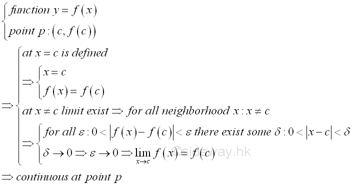
When every point on the domain of function fulfil the Epsilon-Delta limit definition, the curve is continuous within the interval of the domain. Since the curve is continuous, the function f(x) is continuous on the domain of the function also. And therefore a function with non-continuous curve is a discontinuous function. For example, a function f(x) represented by a discontinuous curve with a hole at x=c 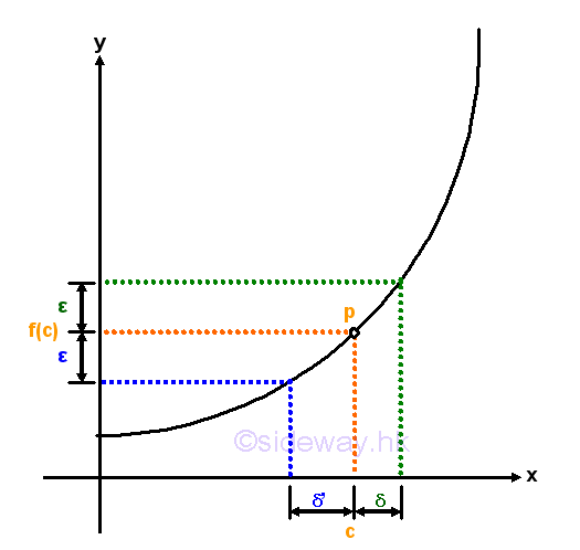
Since the function is not defined at x=c, although the limit at x=c exist, the curve is not continuous at x=c, and the function is not a continuous function also. Or, a function f(x) represented by a discontinuous curve with a gap around x=c. 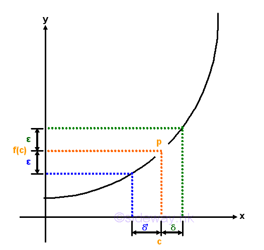
Since the function is not defined around x=c and the limit at x=c does not exist, the curve is not continuous at x=c, and the function is not a continuous function also. Or, a function f(x) represented by a discontinuous curve with a jump at x=c. 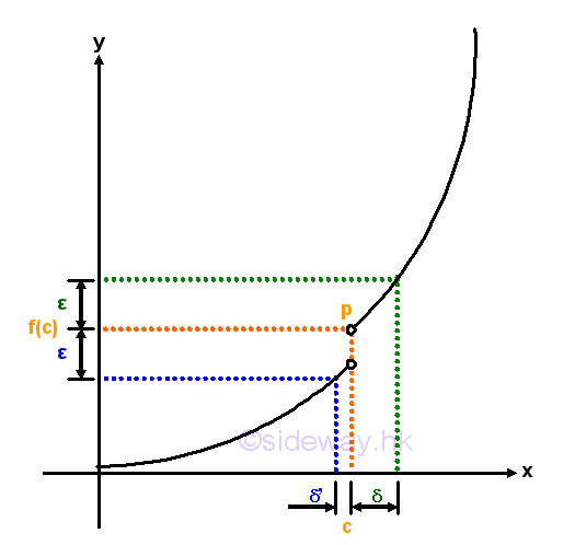
Since the function is not defined at x=c and the limit at x=c does not exist, the curve is not continuous at x=c, and the function is not a continuous function also. Or, a function f(x) which is defined at x=c represented by a discontinuous curve with a jump at x=c. 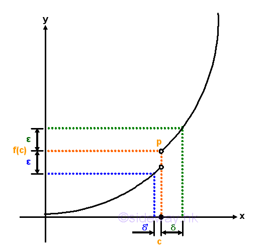
Although the function is defined at x=c, but the limit at x=c does not exist, the curve is not continuous at x=c, and the function is not a continuous function also. Or, a function f(x) which is defined at x=c represented by a discontinuous curve with a hole at x=c. 
Although the function is defined at x=c and the limit at x=c does exist, but the limit at x=c is not equal to the functional value at x=c, the curve is not continuous at x=c, and the function is not a continuous function also. Therefore the curve of a function f(x) is continuous if the functional value at any point c on the domain should be defined, i.e. f(x)=f(c) at x=c and the limit at any point c on the domain does exist and to the functional value at c, i.e. lim f(x)=f(c) at x→c. However, from the above two examples, although a function is defined continuously at x=c, the curve is not continuous and the function is not continuous also. Therefore, a continuously defined function does not imply a function have a continuous curve or the function is continuous. Continuous FunctionFor a function f(x) such that the function of x is defined on the interval a≤x≤b, if for all c such that the limit of f(x) is always exist and equal to f(c) when x approaching c, implying the function f(x) is continuous at x=c, then when the limit taking at x=c is alway valid on the interval a≤c≤b, the function f(x) is continuous in the interval a≤x≤b. Therefore a continuous function is usually defined on an interval. For example, algebraic function is a continuous function on the interal -∞<x<∞. Let f(x)=an. Imply 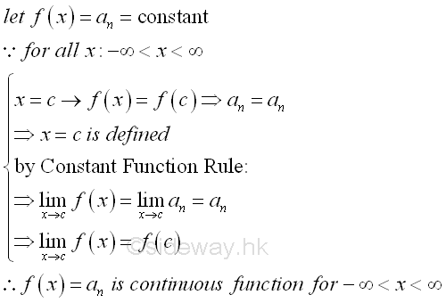
Let f(x)=x. Imply 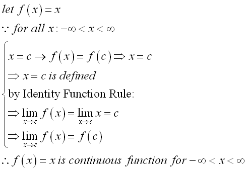
Let f(x)=x2. Imply 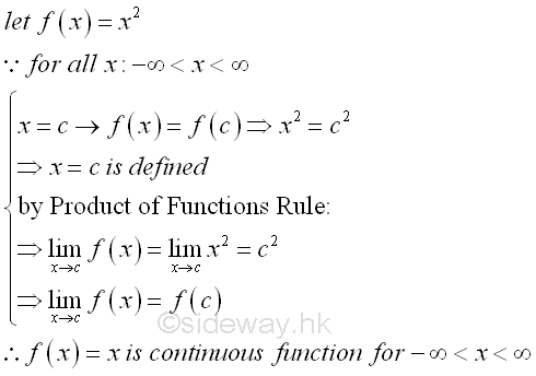
Let f(x)=an-1x. Imply 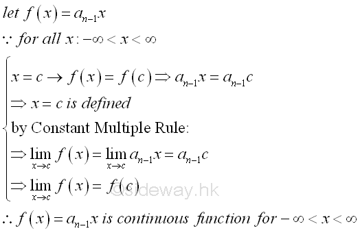
Therefore, by making use of limit of function rules, a rational integral function is continuous function. Imply 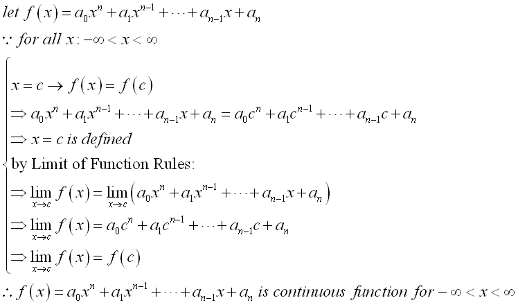
Similarly, by making use of limit of function rules, a rational fractional function is also continuous function. Imply 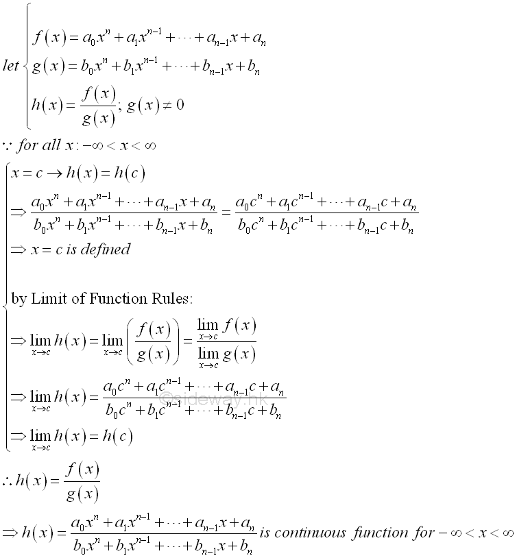
For example, some trigonometric function is a continuous function on the interal -∞<x<∞. Let f(x)=sin x. Imply 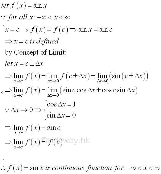
Let f(x)=cos x. Imply 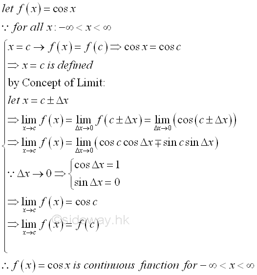
For the exponential function f(x)=ax, where a is a positive number and not equal to 1 is a continuous function on the interal -∞<x<∞. The number a is a positive number because when a is equal to either 0, the exponential function becomes a constant function. Besides, the exponential function also becomes a constant function when a=1. Number a is greater than zero so that there is only real number and no complex root during root extraction. When a is a positive number and x is a rational number, the functional value of the function can be calculated by simple arithematic. And for the root extraction, an exponential function f(x)=ax is usually considered to be a positive function that only the positive roots is considered whenever both the positive and negative roots are possible roots of the function. At x=0, the exponential function f(x)=ax, is equal to one. For any x, the quantiy of the exponential function f(x)=ax will always be greater than zero and in general an exponential function f(x)=ax will never be equal to zero. If a>1, then the ax will increase as x inrease, the exponential function f(x)=ax is an increasing function. If 0<a<1, then the ax will decrease as x increase, the exponential function f(x)=ax is an decreasing function. Since the exponential function ax is an increasing function when a is greater than 1, when rewritting the exponential function in term of (1/a), which is 0<a<1, into an exponential function of (1/a)-x , the rewritten exponential function becomes a decreasing function. Besides the number a, the only difference between two exponential function is the sign of the power. In other words, the increasing function f(x)=ax with a>1 when x →∞ is same as the decreasing function f(x)=ax with a<1 when x →-∞. Therefore if a>1, then when x→∞, ax→∞. and when x→-∞, ax→0. And if 0<a<1, then when x→∞, ax→0, and when x→-∞, ax→∞. As x=0, the exponential function a0=1 is known, the continuity of the exponential function ax at x=1 is 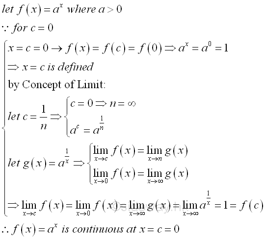
Therefore, the exponential function ax is continuous at x=0. For any rational number x=c, the continuity of the exponential function ax at x=c is 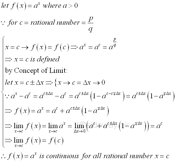
Therefore, the exponential function ax is continuous for all rational numbers. For any irrational number x=c, there always exists a pair of rational numbers such that the irrational number c is bounded when taking limit. The continuity of the exponential function ax at x=c is 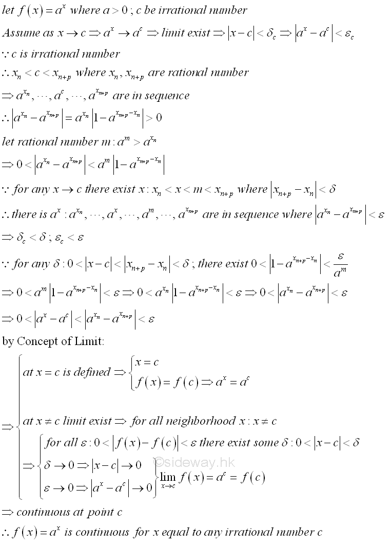
Therefore, the exponential function ax is continuous for all irrational numbers also. Since the exponential function ax is continuous for both rational and irrational numbers, the exponential function ax is a continuous function on the interal -∞<x<∞. The properties of the exponential function f(x)=ax, is 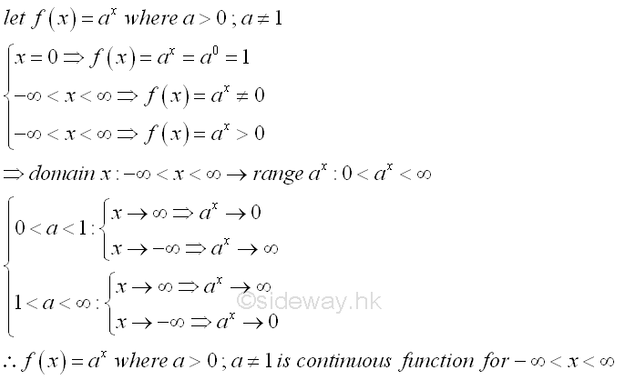
Since logarithmic function y=logax is the inverse function of exponential function x=ay , the Logarithmic function y=logax is a continuous function also. Similarly, number a cannot be equal to 0 and 1, and number a can only be other positive number. Since the range of the exponential function on the domain interval of -∞<x<∞ is equal to the interval 0<y<∞, the domain of the Logarithmic function y=logax can only be on the interval 0<x<∞. While the range of the Logarithmic function y=logax can be on the interval of -∞<x<∞. If a>1, the Logarithmic function y=logax is an increasing function, while if 0<a<1, the logarithmic function y=logax is a decreasing function. The properties of the logarithmic function y=logax , is 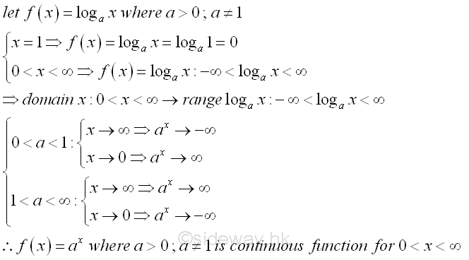
©sideway ID: 130100005 Last Updated: 1/29/2013 Revision: 0 Ref: References
Latest Updated Links
  Nu Html Checker Nu Html Checker  na na |
 Home 5 Business Management HBR 3 Information Recreation Hobbies 9 Culture Chinese 1097 English 339 Travel 45 Reference 79 Hardware 55 Computer Hardware 261 Software Application 213 Digitization 37 Latex 52 Manim 205 KB 1 Numeric 19 Programming Web 289 Unicode 504 HTML 66 CSS 65 SVG 46 ASP.NET 270 OS 431 DeskTop 7 Python 72 Knowledge Mathematics Formulas 8 Set 1 Logic 1 Algebra 84 Number Theory 206 Trigonometry 31 Geometry 34 Calculus 67 Engineering Tables 8 Mechanical Rigid Bodies Statics 92 Dynamics 37 Fluid 5 Control Acoustics 19 Natural Sciences Matter 1 Electric 27 Biology 1 |
Copyright © 2000-2026 Sideway . All rights reserved Disclaimers last modified on 06 September 2019