
|
Draft for Information Only
Content Kinematics:
Three Dimension
Kinematics: Three DimensionIn three dimension, if an object moves linearly in three dimension, the motion of the object can be considered as a rectilinear motion as in one dimension or two dimension. When an object moves along a curve, the object is in curvilinear motion. The position of the object can also be refered to a rectangular coordinate system because the position of an object in space can be described in terms of three dimensional rectangular axes. Since the object moves in a three dimension space, both the direction and magnetude of a vector quatity are needed to be specified. If the object itself does not rotate or change its oreientation or the change can be neglected, the object is under translation motion also, that is the object is shifted along the path in three dimension simultaneously. Vector Functions of MotionPosition Vector FunctionSimilar to one or two dimension, the position of an object at P can be defined by drawing a verctor r from the origin O of a rectangular coordinate system to the positioning point P of the object. Since the vector r can be used to completely define the position of the object by its magnitude r and its direction with respect to the rectangular coordinate system, the verctor r is therefore called position vector of the object. When an object moves along curve, the position of the object can be defined as a vector function r with respect to time t, that is the vector r=r(t) is refered to position P at time t. When the object moves to another position P' after Δt, another position vector r' can be constructed accordingly. Since r is a vector function, position vector r' can be expressed as r'=r(t+Δt). 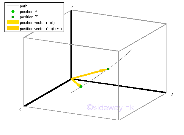
Displacement Vector FunctionThe displacement of the object from position P to P' can be represented by a vector Δr joining points P and P'. In other words, the change in the position vector r during the time interval Δt is equal to the vector Δr, that is r'-r=Δr. As a vector quantity, the vector Δr represents both the change in direction and the change in magnitude. Besides, vector is a fuction of time t also. Since the object is in curvilinear motion, the travelled distance Δs is always not equal to the displacement of the object. 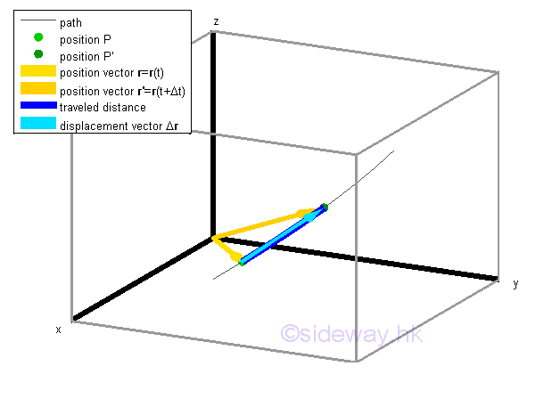
Velocity Vector FunctionBy definition, the average velocity v̅ of the motion over the time interval Δt is equal to the quotient of Δr and Δt. The average velocity of motion is a vector quantity also since the vector quantity Δr is divided by a scalar quantity Δt. The vector v̅ is usually attached to the position P to indicate the beginning of the rate of change with direction same as the displacement vector Δr and with magnitude equal to the magnitude of Δr divided by Δt. Similarly, the average speed s̅ of the motion over the same time interval Δt is equal to the quotient of Δs and Δt. The average speed of the motion is a scalar quantity only since both Δs and Δt are scalar quantities. The average speed is always not equal to the average velocity in curvilinear motion when the time interval is large. 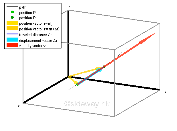
When the time interval Δt becomes shorter and shorter, the positions P and P' becomes closer and closer and the displacement vector Δr becomes shorter and shorter also. As the time interval Δt approaching zero, the displacement vector Δr is also approaching zero and the travelled curvilinear distance Δs becomes closer to the linear displacement Δr. 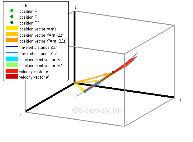
The instantaneous velocity of the object at time t can therefore be obtained by choosing a shorter time interval Δt such that all average velocity of the object obtained during the time interval can be approximated by the average velocity Δr/Δt and the average velocity v̅ can then be used to approximate the intantaneous velocity at position P when taking limit as Δt approaching 0 also. 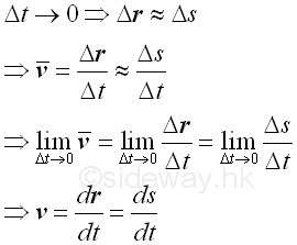
The instantaneous velocity of the object at time t and t+ Δt can therefore be determined accordingly of direction equal to the direction of the displacement vector which is tangent to the path when taking limit and of magnitude equal to the speed which is obtained by differentiating the motion of the object r(t) with respect to time t. 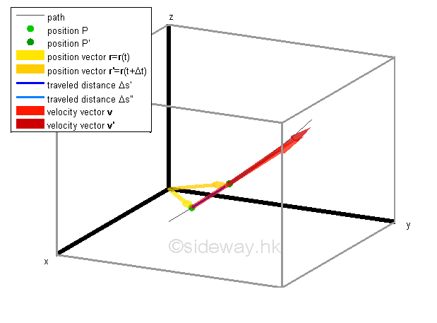
Acceleration Vector FunctionBy definition, the average acceleration a̅ of the motion over the time interval Δt is equal to the quotient of Δv and Δt. The average acceleration of motion is a vector quantity also since the vector quantity Δv is divided by a scalar quantity Δt. The acceleration vector a̅ is usually attached to the position P to indicate the beginning of the rate of change with direction same as the change of velocity vector Δv and with magnitude equal to the magnitude of Δv divided by Δt. Similarly, for curvilinear motion over the same time interval Δt , the average scalar acceleration a̅ of the motion is always not equal to the average vector acceleration a̅ when the time interval is large. And therefore, in general, the acceleration is not tangent to the path unless the motion is a linear motion since acceleration vector a̅ also changes the direction of motion in a curviinear motion also. 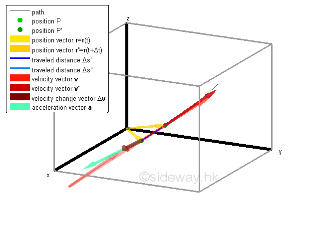
When an object moves continuously along a path, the motion of the object can also be plotted according its velocity v with respect to the time t instead of according to its position. If the velocity v changes continuously, a smooth curve can be ploted on a rectangular coordinate system with magnitudes of axes representing the dimensions of velocity along the position axes, not position, also. The curve drawn from the intantaneous velocity v is called hodograph of the motion which indicate the rate of change of the velocity of the motion with respect to time, not position. For example, at time t, the velocity of the object is equal to Q and is represented by a velocity vector v=v(t), after time interval Δt, the velocity of the object is equal to Q' and is represented by a velocity vector v'=v(t+Δt). 
Similar to displacement, the change in the velocity of the object with respect to time during the time interval Δt can be represented by a vector Δv which represent both the direction and magnitude of the change in velocity. The average acceleration a̅ of the motion over the time interval Δt which is equal to the quotient of Δv and Δt, can be obtained similarly. The average acceleration of motion is a vector quantity also since the vector quantity Δv is divided by a scalar quantity Δt. The vector a̅ is usually attached to the position Q to indicate the beginning of the rate of change with direction same as the change in velocity vector Δv and with magnitude equal to the magnitude of Δv divided by Δt. 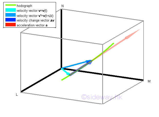
When the time interval Δt becomes shorter and shorted, the rate of change in velocity during the time interval Δt becomes more linear also. 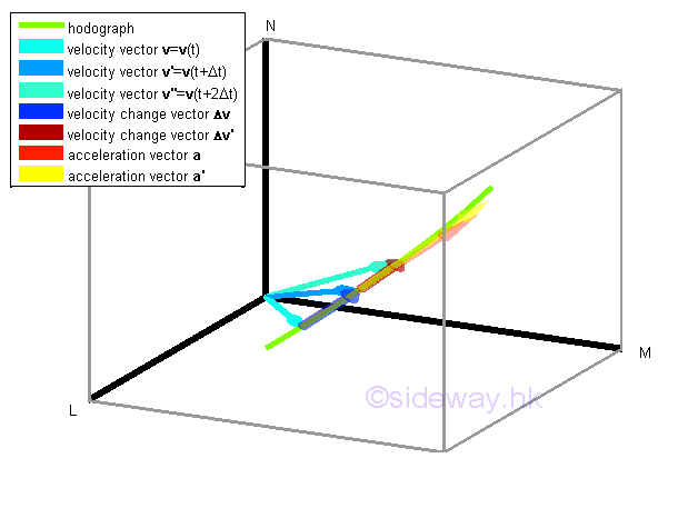
The instantaneous acceleration of the object at time t can therefore be obtained by choosing a shorter time interval Δt such that all average acceleration of the object obtained during the time interval can be approximated by the average acceleration Δv/Δt and the average acceleration a̅ can then be used to approximate the intantaneous acceleration at time t when taking limit as Δt approaching 0 also. 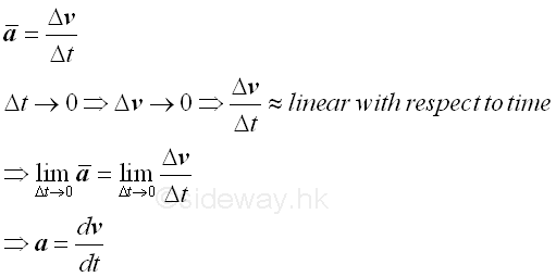
The instantaneous acceleration of the object at time t and t+ Δt can therefore be determined accordingly of direction equal to the direction of the change in velocity vector which is tangent to the curve of the hodograph of motion, not the path, when taking limit and of magnitude equal to the acceleration which is obtained by differentiating the motion of the object v(t) with respect to time t. 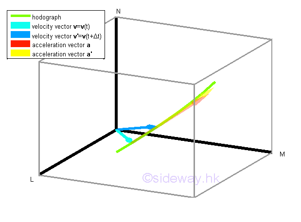
Unlike rectilinear motion, in general, the velocity or the intantaneous velocity is tangent to the path of the object in curvilinear motion and the acceleration in not tangent to the path of the object unless the object is in linear motion instantaneousl. 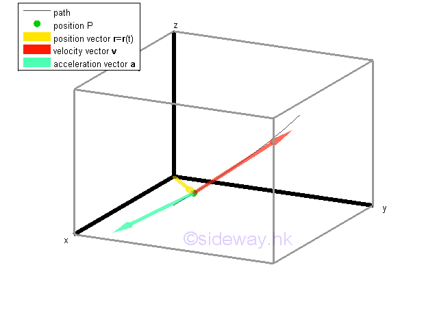
©sideway ID: 140300005 Last Updated: 6/17/2014 Revision: 1 Ref: References
Latest Updated Links
  Nu Html Checker Nu Html Checker  na na |
 Home 5 Business Management HBR 3 Information Recreation Hobbies 9 Culture Chinese 1097 English 339 Travel 45 Reference 79 Hardware 55 Computer Hardware 261 Software Application 213 Digitization 37 Latex 52 Manim 205 KB 1 Numeric 19 Programming Web 289 Unicode 504 HTML 66 CSS 65 SVG 46 ASP.NET 270 OS 431 DeskTop 7 Python 72 Knowledge Mathematics Formulas 8 Set 1 Logic 1 Algebra 84 Number Theory 206 Trigonometry 31 Geometry 34 Calculus 67 Engineering Tables 8 Mechanical Rigid Bodies Statics 92 Dynamics 37 Fluid 5 Control Acoustics 19 Natural Sciences Matter 1 Electric 27 Biology 1 |
Copyright © 2000-2026 Sideway . All rights reserved Disclaimers last modified on 06 September 2019